Work Log – Urmila Chadayammuri

Primer: The Sunyaev-Zel’dovich Effect

April 16, 2018uc24 Leave a Comment

Galaxy cluster RX J1347.5-1145 observed with ALMA (blue) and HST (background)

The Sunyaev-Zel’dovich effect is this really really awesome process that allows us to see clusters of galaxies at all distances. It is going to be vastly important with all the fancy new submillimeter telescopes astronomers have built lately, such as the Atacama Large Millimeter Array (ALMA), the Sub-Millimeter Array (SMA) and the Atacama Cosmology Telescope (ACT). At its core, it’s a beautifully simple phenomenon, so let’s break it down.

About 10% of the mass of galaxy clusters is intra-cluster gas, not attached to any individual galaxy. To counter the strong gravitational potential of the dark matter with thermal pressure, the gas needs high temperatures of 1-100 million Kelvin. Gas this hot is best observed with X-ray telescopes.

Light from the cosmic microwave background (CMB) is coming at us from all directions. Since these photons started out ~13 billion light years away from us, when light and matter separated for the first time, they pass through plenty of galaxy clusters on their way to us. And when they hit the very hot electrons in the ionized intra-cluster gas, they get “upscattered” – that is to say, they get more energy, while the electrons cool down a tiny bit. This is called inverse Compton scattering; in regular Compton scattering, the photon would have been hotter than the electron, so the energy transfer would have gone the opposite way.

A photon Compton scatters against an electron, gaining some energy and sending the electron into a slight recoil.

The magnitude of cooling due to the SZ effect is:

$\frac{\Delta T}{T_{CMB}} = f(x)\int \sigma_T n_e \frac{kT_e}{m_ec^2}dl$

where x = $\frac{h\nu}{k_BT_{CMB}}$ describes how this cooling depends on the rest frame frequency $\nu$ that you observe. In words, it is the integral along the line of sight of the thermal pressure of the electrons normalised by the rest energy of electrons, all multiplied by the Thomson cross-section, which sets the scale of the photon-electron interaction. This quantity is called the SZ decrement.

Okay now are you ready for the coolest (IMHO) bit? Consider how the value of the SZ decrement varies with redshift/distance. Since the Universe was (1+z) times smaller in each dimension at a redshift z, the number density of a cluster with a given total number of electrons goes as:

$n_e = \frac{3 N_e}{4\pi r^3}$ $=\frac{3 N_e}{4\pi r_0^3} (1+z)^3$

Meanwhile, that line element dl that we’re integrating over can be written as:

$dl = \frac{dr^3}{d_A^2} = \frac{dx^3}{d_L^2}\frac{ (1+z)^2}{(1+z)^3}$

where, $d_A$ is the angular diameter distance and $d_L$ the luminosity distance. Following the same expansion argument as above, each of those dimensions was (1+z) times smaller, giving a total dependence of (1+z). So the intrinsic/rest frame SZ decrement increases with redshift as $(1+z)^4$ .

Now the energy density from a source at redshift z decreases as $(1+z)^3$ due to cosmological expansion, plus a $(1+z)$ fall-off in the frequency. This means that an object of a fixed luminosity L gets $(1+z)^{-4}$ times fainter with redshift.

The redshift dependences of the SZ decrement and fading due to distance exactly cancel out!

This means that given a mass of a cluster (and thus $N_e$ ), we can detect it with the SZ effect at every redshift ever. It’s a redshift-independent tracer of mass. It means that we can study the assembly history of massive objects in the Universe to as far out as we freaking want, as long as the temperature measurements are precise enough! And currently, they are enough to see anything upwards of about $10^{14}M_\odot$ .

#Sparknotes: Black Holes as Chaotic Eaters

September 1, 2016uc24 Leave a Comment

Chaotic cold accretion onto black holes

Gaspari, Ruszowski and Oh, 2013

This paper describes a set of very high resolution, idealized simulations of a supermassive black hole (SMBH) in the central (cD) galaxy of a massive cluster. Since the goal is essentially to challenge the current near-universal use of the Bondi accretion model in simulations, let’s start with the key equation:

Setup Start with a simple NFW dark matter halo, a de Vaucouleurs stellar distribution, gas that traces the gravitational potential and a SMBH, all with masses similar to the observed galaxy group NGC 5044. All of these are modelled in an adaptive mesh grid overlaid on a box of side 52kpc for a total time of 40 Myr. With upto 44 levels of refinement, the simulation resolves sub-parsec scales around the central black hole.

Mass accretion onto the black hole, normalized by Bondi prediction.

Varying physics models

The initial setup thus consists of an ideal gas contracting under gravity. This results in adiabatic, isotropic, smooth accretion of warm gas, identical to the analytic model of Bondi (1952). Indeed, the (numerically) observed accretion in this case exactly matches Bondi’s prediction, since the solid line in Fig 1b is essentially = 1 throughout. What is the dashed line, you ask? Well, that is the accretion rate you would measure if you evaluated the parameters in the Bondi equation as an average over a cluster-centric radius of 1-2 kpc, instead of at the Bondi radius (85pc in this case). In other words, computing gas density and sound speed as an average over large cells overestimates the accretion rate.

The simulations sequentially complicate the physics.

First they add cooling, which occurs due to atomic transitions in the ICM. Observed cluster ICMs tend to be quite enriched in metals, mostly due to ejecta from supernovae. They assume the metallicity of the cluster gas to equal that of the sun, which I thought was generous but is actually supported by Chandra observations (e.g. Vikhlinin et al 2005). The accretion is now boosted by over two orders of magnitude. Of course, the simulation doesn’t model star formation; if it did, a lot of this centrally accreted gas could actually be converted into stars, so we would observe very large star formation rates in over very short time scales in the central galaxies of clusters. We d not.

Next, they add turbulence by “stirring” the gas on large scales (lol 4kpc; this is just about the resolution of our cosmological simulation. It’s so relieving to see that someone is actually probing the smaller regions so that our sub-grid models aren’t full of hot air.)(I’m sorry I can’t help these things.) In reality turbulence can be induced by galaxy motions through the viscous ICM, galaxy-galaxy mergers, AGN and stellar feedback, etc. And this is where things start to look really different.

You now see a slice of the temperature profile of the gas. Adding the metal cooling, as mentioned above, decreases the temperature in the core by over 4 orders of magnitude, but retains the spherical symmetry and isotropy. Adding turbulence creates very cold filaments on very large scales. The accretion is on average as high as in the cooling-only scenario, but with more fluctuations.

Lastly, they consider global heating. In a real cluster, this could come from cosmic rays, AGN feedback, massive stellar feedback, etc. This suppresses the star formation somewhat from the previous case, but the “boost factor” with respect to the Bondi prediction is just under 100 by the end of the simulation. The filaments induced by turbulence are not broken up or significantly heated up.

In summary: accretion of gas onto the supermassive black holes at the centres of galaxy clusters is cold, chaotic and filamentary. Averaged over tens of megayears, the boost factor with respect to the Bondi model is just under 100, compared to the prevalent norm of 100-400.

#Sparknotes: AGN

August 15, 2016uc24 Leave a Comment

So excited about this fall! I get to implement a new subgrid model for accretion onto, and feedback from, active galactic nuclei (AGN) at the centres of clusters in a cosmological simulation we develop here at Yale.

Developing subgrid models (and numerical approximations in general) is an art as much as a science. On the one hand, you need to reproduce large-scale, observable phenomena, like star formation histories, stellar masses, stellar and metallicities, and dark and visible substructure. On the other, you want your input parameters to be motivated by plausible underlying physics.

Fig 1 from Urry and Padovani, 1995

AGN are a pesky beast. They consist of a supermassive black hole (SMBH) at the core, or nucleus, of a galaxy, surrounded by a hot disk of infalling matter. Since the material in the disk is unlikely to have falling in on a radial trajectory, it settles in a rotating disk around the black hole. Friction between layers of the disk heat it up to tens of millions of Kelvin, so that if you catch an AGN at the correct angle, it is bright in the X-ray. More often than not, due to geometric reasons, you’ll end up seeing dust-obscured AGN, which are bright in the radio. That’s a two-line summary of the Unified Model of AGN.

This obscuration, combined with the final parsec problem, is the main reason AGN are so pesky. Stuff falls onto black hole, aggravates it, isothermal heat ejections and mechanical jets arise! But what sort of stuff can fall into the black hole? Why does that cause it to spit stuff out? How exactly does it eject this energy? How far does the energy travel, and how does it interact with gas on its way (more specifically, the Intra-Cluster Medium or the ICM)?

There has been a sea of observations and theoretical models on this topic in the last few decades, and I’m just starting to dip my toes in it. Here’s a summary of the papers I’ll review in the next months.

How is energy transported within an accretion disk? How do the viscosity, density and temperature of the gas in the accretion disk determine whether energy transport is dominated by radiation, advection or convection? What does each of these processes look like? Advection-Dominated Accretion around Black Holes – Narayan, Mahadevan and Quataert, 1998
How exactly does the gas fall onto the black hole? How cold does it have to be? Does this depend on whether the gas is in filaments or clouds, and how those may be oriented? Growing supermassive black holes by chaotic accretion – Gaspari et al, 2013
The simulation I work with extracts clusters of galaxies from a cosmological box. This captures things idealized/isolated cluster simulations cannot, like smooth accretion of gas from filaments and mergers of clusters. Accretion during the merger of supermassive black holes – Armitage and Natarajan, 2002
Several self-regulating mechanisms have resulted in tight relations between galaxies and the supermassive black holes that live in their centres. Accreting supermassive black holes in the COSMOS field and the connection to their host galaxies – Bongiorno et al, 2012.
- Also, Self-regulated Growth of Supermassive Black Holes in Galaxies as the Origin of the Optical and X-Ray Luminosity Functions of Quasars – Wyithe and Loeb, 2003

Yale Frontier Fields Workshop 2014

November 17, 2014uc24 Leave a Comment

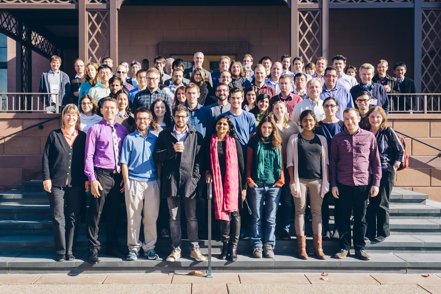
A year after the launch of the Hubble Frontier Fields, my supervisor Priya Natarajan and Dan Coe at the Space Telescope Institute (STScI) in Baltimore put together the first science meeting of the sizable collaboration. Celebrity attendants included Matt Mountain, Director of STScI, Mark Postman, PI of the Cluster Lensing And Supernova survey with Hubble (CLASH) mission and Neta Bahcall – professor at Princeton, long-time project leader at STScI and general cosmology legend.

YFF 2014

Most of the presentations are available here. Talks fell broadly into three categories:

Observations with the Hubble Frontier Fields, i.e. studies of the baryonic physics of galaxies and galaxy clusters. These were often combined with observations in the X-ray from Chandra and in the infrared from Subaru, as also with spectroscopy from MUSE (which was a source of much excitement). These were used to probe the faint end of various mass and luminosity functions, as well as high-redshift objects which were magnified by the cluster lenses.
Lensing reconstructions of the substructure of the HFF clusters (the project currently targets six clusters and six parallel fields), i.e. studies of large-scale structure and tests of cosmological models. Combined strong and weak lensing maps have been completed for Abell 2744 using parametric as well as free-form lensing models; MACS 0416 has been modeled using strong-only constraints under the same two schemes. I got to plot these results against the demographics of the Illustris universe, an exciting result which should make it to paper form within a couple months. A bit more on my favourite talk in this category below.
Panels on the history and direction of large observation projects, i.e. how to do science. Gus Evrard in particular spoke to my heart when arguing for the importance of accessible simulations and their application in identifying systematic errors in various observation schemes. Incidentally, the Illustris Project has just released its first virtual observatory!!! We just may have convinced the admin folk at STScI of the necessity for many more funds in the area of computation to correctly interpret the observations from the massive surveys of this age – the recently completed SDSS and DES, the ongoing HFF and of course the upcoming mammoth that is the JWST.

The highlight for me was definitely Massimo Meneghetti’s closing talk describing a lensing method comparison project. Massimo works at the Bologna Lens Factory (BLF), commissioned by ESA’s Euclid mission to generate a suite of simulated galaxies and clusters against which to test lensing reconstruction tools. An ongoing project has been asking various teams to reconstruct the dark matter substructure in two simulated clusters from BLF, and comparing them to the known, true configuration. A joint paper summarizing the systematics of various methods should be out sometime over the next year as people tweak their models to their satisfaction.

All in all, epic time 🙂 It was pretty amazing to see such genuine curiosity and generous sharing of data and methods. Coming from a background primarily in theory, I used to think of error bars as a painful formality – but the statistical tests of cosmological models we and others performed and presented last week have got me positively nerding out about these. Good science should know exactly what it doesn’t know as well as what it does.

To collaboration and humility! And funding for theory.

Python rules and a conference

July 11, 2014uc24 Leave a Comment

Tired to the bones from 9 hours on a bus and 5 hours of solid discussion. Totally worth it.

Turns out I don’t need dozens of packages to analyze Gadget, or for that sake AREPO, output. The team has put together a bunch of Python scripts to read and visualize this in a myriad of ways, so I just need to work through a comprehensive Wiki to get familiar with the methods.
Got the output of an existing simulation run to get the hands dirty in analysis without worrying about execution errors in the code itself.
Teams at Heidelberg and Cambridge are already running the simulations needed for my analysis and should be done in a couple weeks, just in time for me to figure out how to analyze the results.
Sat in on a presentation of rotational variations between various regions of galactic halos in circular versus elliptical galaxies. The angular velocity distribution of stars within a halo appears to be much more skewed for circular galaxies, which in turn are understood as having remained stable (accretion/merger-free) for a longer time. This led to a discussion of various sources of alignment or, conversely, counter-rotation. Not my focus, but something to consider when working with cluster merger simulations in the future.
There is an invitation-only seminar at the American Association for Arts and Science in Cambridge the first week of September and I get to make a presentation! Something concrete to work towards = extra exciting.

The upcoming weeks, then, will be all about getting comfortable with the analytical scripts already developed in Python. There’s also a mini-reunion of various alum of the lab a week from now, leading to more fun presentations and rooftop chats.
Oh and GRE prep. I should really do that.

Gadget and fluid dynamics

July 10, 2014uc24 Leave a Comment

This week was mostly installing packages.

The simulations I’ll be working on in the nearest future use AREPO, a hydrodynamic simulation code.
A good introduction, and the primary tool in later work, is the Gadget code.
The output is a series of snapshots, which need to be compiled into a video for meaningful interpretation. This requires GadgetViewer, a visualization software.
Running this, in turn, asks for GTK+ 2.0, a tool for creating graphical user interphases.
Given the multiple languages used across these packages, I also had to install gettext, an open-source utility that structures other programs such that every function therein knows where to look for certain necessary files (mostly libraries and commands).

Yup, that’s a lot of packages.
And of course files are located in weird places, some are remotely accessed.. So making sure everything installs correctly is a much larger task than I would have thought. Not really complaining though – I can see myself getting better reading and editing source code by the hour.
Meanwhile, I’d also obviously like to understand the physics behind these simulations and how they compare with alternatives. This is quite alien to the fluid mechanics noob that I am.

AREPO uses the numerical Godunov scheme to model fluid behaviour on a moving mesh, in contrast to the analytical approach taking in both Eulerian and Smoothed Particle Hydrodynamics (SPH). The two of these in turn differ in how they look at the system.
The Eulerian approach considers conservation of certain properties, namely momentum and energy, and continuity of mass within a region of space. The Godunov scheme in fact builds on Eulerian conservation laws. Pre-AREPO, however, simulations would consider these dynamics on a Cartesian plane, resulting in a loss of Galilean invariance (the requirement that laws of motion be the same in all inertial frames). How exactly? That, and how AREPO’s moving mesh handles the issue, are questions for a future post when I know better.
SPH, as the name indicates, follows the dynamics of each constituent particle (or fluid elements, rather), in turn dependent on the properties of others surrounding it. This smoothing, however, mutes the effect of instabilities within the smoothing length. Turbulence can have significant effects on thermal and magnetic pressure (depending on whether the fluid studied is a gas or a magnetic field), as noted in Lage’s recent paper modeling a merger in the Bullet cluster, where he had to introduce a physically unknown fudge factor to maintain gas clouds in equilibrium.

I’ll be digging some brains at the CfA tomorrow, attending lab meeting and mapping out a project sequence with my immediate supervisor. All good things.